Women's College Basketball Player Value: Box Plus-Minus Model

Box plus-minus (BPM) estimates a player’s contribution in points per 100 possessions from her box score alone: scoring, efficiency, usage, rebounding, assists, steals, blocks and turnovers. It cannot see screens, spacing or defensive positioning, but because box score rates settle quickly it is far more stable than on/off measures at college sample sizes. load_wbb_player_value() returns offensive, defensive and total BPM for every Division I women’s player since 2014.

This article explains what the model estimates, how it is fitted, how it holds up, and how to use it responsibly. It condenses the official model card in the wehoop-wbb-data repository; numbers quoted from that card are labelled as such.

What the model estimates

Column	Meaning
`box_obpm`	Offensive box plus-minus, points per 100 possessions above average
`box_dbpm`	Defensive box plus-minus
`box_bpm`	`box_obpm + box_dbpm`
`min`	Minutes played
`qualified`	`TRUE` when `min >= 300`, the floor below which the estimates are mostly noise
`player_id`, `player`, `team_id`, `season`	Identifiers (ESPN ids)

BPM and RAPM measure different things. RAPM (see the women’s college RAPM article) sees everything that happens while a player is on the court but needs many possessions. BPM sees only the box score but needs few. Treat them as cross-references, not substitutes.

Loading the ratings

The ratings are published as Parquet files, so load_wbb_player_value() needs the arrow package.

library(wehoop)
library(dplyr)
library(ggplot2)

pv <- load_wbb_player_value(seasons = 2025:2026)

# Older release files predate the `qualified` flag; derive it the same way.
if (!"qualified" %in% names(pv)) pv$qualified <- pv$min >= 300

pv |> count(season, qualified)
#> # A tibble: 4 × 3
#>   season qualified     n
#>    <int> <lgl>     <int>
#> 1   2025 FALSE      4921
#> 2   2025 TRUE       2920
#> 3   2026 FALSE      5293
#> 4   2026 TRUE       3012

Team names come from the box scores, joined on character ids:

team_names <- load_wbb_team_box(seasons = 2026) |>
  transmute(team_id = as.character(team_id), team = team_location) |>
  distinct(team_id, .keep_all = TRUE)

pv <- pv |>
  mutate(team_id = as.character(team_id), player_id = as.character(player_id)) |>
  left_join(team_names, by = "team_id")

pv |>
  filter(season == 2026, qualified) |>
  arrange(desc(box_bpm)) |>
  select(player, team, min, box_obpm, box_dbpm, box_bpm) |>
  mutate(across(where(is.double), ~ round(.x, 2))) |>
  head(15)
#> # A tibble: 15 × 6
#>    player          team             min box_obpm box_dbpm box_bpm
#>    <chr>           <chr>          <dbl>    <dbl>    <dbl>   <dbl>
#>  1 Jana El Alfy    UConn            402     6.7     11.4     18.1
#>  2 Kyla Oldacre    Texas            830    10.4      7.54    17.9
#>  3 Madina Okot     South Carolina   906    10.6      6.86    17.4
#>  4 Sarah Strong    UConn           1044    15.8      1.61    17.4
#>  5 ZaKiyah Johnson LSU              642    11.0      5.41    16.4
#>  6 Lauren Betts    UCLA            1026    15.3      0.83    16.2
#>  7 Amiya Joyner    LSU              709     8.22     7.86    16.1
#>  8 KK Arnold       UConn            928     5.01    10.7     15.7
#>  9 Kate Koval      LSU              582     8.37     7.27    15.6
#> 10 Anaya Hardy     Louisville       399     9.09     6.49    15.6
#> 11 Grace Knox      LSU              611     9.59     5.76    15.4
#> 12 Mir McLean      Maryland         463     6.9      8.39    15.3
#> 13 Kiki Rice       UCLA            1170    10.8      4.21    15.0
#> 14 Teya Sidberry   Texas            487     5.33     9.7     15.0
#> 15 Raegan Beers    Oklahoma         843    13.3      1.7     15.0

Data

As reported in the model card, the inputs are the published player and team season statistics for women’s college basketball, and the team ratings from load_wbb_ratings(). Coverage starts in 2014, the first season with box score inputs of sufficient quality. The model is recomputed from the current published data on every run, so upstream corrections flow through on the next publish.

How the model works

Per-100 features. Each player’s box score is converted to rates per 100 possessions and shares: points, assists and rebounds per 100, usage, true shooting and effective field goal percentage, turnover, steal, block, assist and rebound percentages, free throw rate, and shot-location shares.
Standardize. Each feature is centered and scaled (and clipped at 4 standard deviations, as reported in the card).
Score. Separate ridge regressions for offense and defense, fitted at the team level, turn the standardized features into raw offensive and defensive scores.
Team adjustment. A uniform adjustment per team makes the team’s minutes-weighted player scores add up to its adjusted efficiency margin from the team ratings model. This is what anchors BPM to winning.

As reported in the model card, the current coefficients were fitted on the 2025 and 2026 seasons with a ridge penalty of 3.0 for both offense and defense and a 150-minute floor for the team-sum weights. Because every feature is standardized, a slope is the BPM change for a one-standard-deviation move in that feature. The largest weights in the card:

Feature	Offense slope	Defense slope
Points per 100	6.932	-5.442
Usage	-4.567	2.661
True shooting %	-0.358	1.818
Rebounds per 100	0.025	1.312
Assists per 100	1.112	-0.877
Turnover %	-0.183	-0.908

The scoring group (points, usage, shooting) carries most of the offensive weight, and the defensive slopes mirror it with flipped signs. That is the team constraint at work: offense and defense must add up to one team rating, so a feature that buys offense is charged against defense. Rebounding and steals are the clearly defensive contributors. The card reports that the coefficient vector is published alongside the release as wbb_player_value_coefficients.json.

How well does it work?

The minutes funnel: why the `qualified` flag exists

The published file keeps every player, including those with a handful of minutes. With no shrinkage, the most extreme values belong to the smallest samples:

pv_2026 <- pv |> filter(season == 2026)

ggplot(pv_2026, aes(min, abs(box_bpm))) +
  geom_point(alpha = 0.15, color = "#221A4D") +
  geom_vline(xintercept = 300, linetype = "dashed", color = "#b298dc") +
  labs(
    title = "Low-minute players produce the most extreme BPM values",
    subtitle = "Dashed line: the 300-minute qualified floor",
    x = "Minutes", y = "|Box BPM|",
    caption = "Data: wehoop::load_wbb_player_value(seasons = 2026)"
  ) +
  theme_minimal()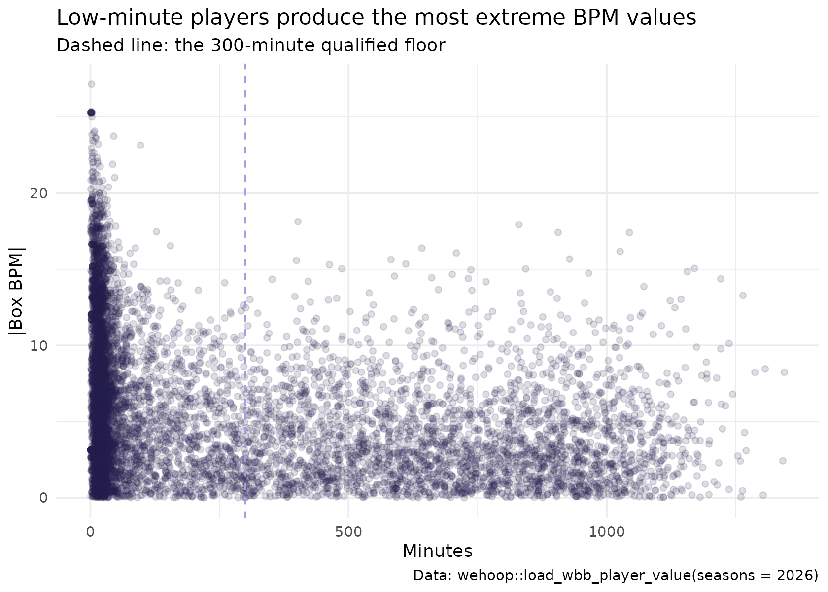

Scatter plot of 2025-26 NCAA women's players: minutes played against absolute box plus-minus; extreme values concentrate at low minutes, with a vertical line at 300 minutes.

pv_2026 |>
  mutate(minutes_bin = cut(min, c(0, 50, 100, 200, 300, 600, 800, Inf),
                           include.lowest = TRUE, right = FALSE)) |>
  group_by(minutes_bin) |>
  summarise(players = n(), sd_box_bpm = sd(box_bpm, na.rm = TRUE), .groups = "drop")
#> # A tibble: 7 × 3
#>   minutes_bin players sd_box_bpm
#>   <fct>         <int>      <dbl>
#> 1 [0,50)         3825       7.38
#> 2 [50,100)        558       6.18
#> 3 [100,200)       509       5.59
#> 4 [200,300)       401       5.04
#> 5 [300,600)      1085       5.01
#> 6 [600,800)       745       4.71
#> 7 [800,Inf]      1182       4.86

The spread of BPM shrinks as minutes rise and levels off. As reported in the model card, the 300-minute floor is the first bin whose spread sits within 2% of the plateau reached at 600 to 800 minutes, measured over all published seasons. Filter on qualified before ranking or comparing players.

Is it stable from season to season?

A box score model earns its place by persisting for returning players. Here is the correlation of BPM from 2025 to 2026 for players qualified in both seasons:

yoy <- pv |>
  filter(qualified) |>
  select(player_id, season, box_bpm) |>
  tidyr::pivot_wider(names_from = season, values_from = box_bpm,
                     names_prefix = "bpm_", values_fn = mean) |>
  filter(!is.na(bpm_2025), !is.na(bpm_2026))

yoy |> summarise(players = n(), yoy_correlation = cor(bpm_2025, bpm_2026))
#> # A tibble: 1 × 2
#>   players yoy_correlation
#>     <int>           <dbl>
#> 1    1533           0.813

As reported in the model card, the same check pooled over every published season pair gives 0.818 over 14,608 player pairs.

Do offense and defense carry different information?

pv_2026 |>
  filter(qualified) |>
  summarise(players = n(), cor_obpm_dbpm = cor(box_obpm, box_dbpm))
#> # A tibble: 1 × 2
#>   players cor_obpm_dbpm
#>     <int>         <dbl>
#> 1    3012       -0.0536

A correlation near zero means the two components are not restating each other.

Reproducing it yourself

Ratings: load_wbb_player_value(seasons = ...) (needs arrow), 2014 onward.
Inputs: load_wbb_player_box() for the box scores and load_wbb_ratings() for the team margins the adjustment uses.
Method and evaluation in full: the model card.

Limitations

The box score is all it sees. Screening, help defense, spacing and defensive attention are invisible, which hurts defensive specialists and helps high-volume scorers.
No shrinkage. Low-minute values are unreliable; use the qualified flag.
Team-anchored. A player’s BPM inherits her team’s adjusted margin, so an error in the team rating moves the whole roster. As reported in the cards, the 2015 team ratings are missing, which leaves every 2015 player value empty.
Not yet blended with RAPM. As reported in the card, a hybrid that uses BPM as a prior for RAPM is the planned next step.

Where to go next

Women’s college RAPM: the on/off counterpart.
Women’s college team ratings: the team margins BPM is anchored to.
WNBA player impact: BPM, SPM and RAPM side by side for the WNBA.
Advanced metrics: the per-100 rates and shooting percentages BPM is built from.
Model dataset loaders in the function reference.

Citation

@misc{wehoop_wbb_player_value,
  author = {Saiem Gilani},
  title = {Women's College Basketball Player Value Model},
  url = {https://wehoop.sportsdataverse.org/articles/womens-college-basketball-player-value-model.html},
  year = {2026}
}

Saiem Gilani