Women's Basketball Advanced Metrics in R: Possessions, Pace, Ratings and the Four Factors

Box score totals reward teams that play fast and players who play a lot. Advanced metrics strip those effects out by measuring per possession and per shot. This article computes the standard set (possessions, pace, offensive and defensive rating, the four factors, effective field goal percentage, true shooting and usage) from the season box scores that wehoop publishes, with every formula written out as dplyr code you can read and change.

Everything here runs offline on pre-built release files, so it is quick and does not touch a live API. If you are new to wehoop, start with Getting Started, whose glossary defines each term.

What you’ll learn

How to estimate possessions from a box score, and how good the estimate is.
How to compute pace, offensive, defensive and net rating.
How to compute Dean Oliver’s four factors for offense and defense.
How to compute eFG%, TS% and usage rate for players.
How the same code runs on women’s college basketball.

wehoop does not ship helper functions for these formulas, so we write them out. That is deliberate here: seeing the formula is the point.

library(wehoop)
library(dplyr)
library(ggplot2)

Load the box scores

We use the 2025 WNBA regular season (season_type == 2).

team_box <- load_wnba_team_box(seasons = 2025) |>
  filter(season_type == 2)
player_box <- load_wnba_player_box(seasons = 2025) |>
  filter(season_type == 2)

ESPN files the All-Star Game as a regular-season game between two one-off teams. Keep only the franchises, which each played a full schedule.

franchises <- team_box |>
  count(team_id) |>
  filter(n >= 20) |>
  pull(team_id)

team_box <- team_box |> filter(team_id %in% franchises)
player_box <- player_box |> filter(team_id %in% franchises)

length(franchises)
#> [1] 13

Possessions

A possession ends when the team on offense makes a shot, loses the ball, or the defense rebounds a miss. Box scores do not count possessions, so we estimate them:

$\text{Poss} = \text{FGA} - \text{OREB} + \text{TOV} + 0.44 \times \text{FTA}$

Field goal attempts start possessions, offensive rebounds extend one (so they are subtracted), turnovers end one without a shot, and 0.44 converts free throw attempts to the trips to the line that end a possession (a two-shot foul is one trip; and-ones and technicals are not trips).

Use total_turnovers, which includes team turnovers such as shot-clock violations; turnovers counts only those charged to a player.

Each team-game row needs its opponent’s stats too (for defensive measures), so join each row to its mirror row from the same game.

games <- team_box |>
  transmute(
    game_id, team_id, team = team_abbreviation, team_score,
    fga = field_goals_attempted, fgm = field_goals_made,
    fg3m = three_point_field_goals_made, fg3a = three_point_field_goals_attempted,
    fta = free_throws_attempted, ftm = free_throws_made,
    oreb = offensive_rebounds, dreb = defensive_rebounds,
    tov = total_turnovers,
    poss = fga - oreb + tov + 0.44 * fta
  )

games <- games |>
  inner_join(
    games |> rename_with(~ paste0("opp_", .x), -game_id),
    by = "game_id",
    relationship = "many-to-many"
  ) |>
  filter(team_id != opp_team_id)

games |>
  select(game_id, team, poss, opp_team, opp_poss) |>
  head()
#> # A tibble: 6 × 5
#>     game_id team   poss opp_team opp_poss
#>       <int> <chr> <dbl> <chr>       <dbl>
#> 1 401736394 NY     76.5 CHI          78.3
#> 2 401736394 CHI    78.3 NY           76.5
#> 3 401736395 PHX    78.5 DAL          81.8
#> 4 401736395 DAL    81.8 PHX          78.5
#> 5 401736396 GS     78.6 MIN          74.0
#> 6 401736396 MIN    74.0 GS           78.6

The two teams’ estimates in a game differ slightly, because the formula is an approximation. A common refinement averages them so both teams share one possession count.

How good is the estimate?

The WNBA Stats API play-by-play lets you count possessions directly. load_wnba_stats_possessions() publishes one row per counted possession from a GitHub release, so we can compare the box score estimate with the count. The two sources use different game ids, so compare the league average per team-game rather than game by game.

counted <- load_wnba_stats_possessions(seasons = 2025) |>
  # regular-season WNBA Stats game ids start with "102"
  filter(substr(game_id, 1, 3) == "102", count_as_possession == TRUE)

poss_check <- tibble(
  source = c("Box score estimate", "Counted from play-by-play"),
  possessions_per_team_game = c(
    mean(games$poss),
    nrow(counted) / (2 * length(unique(counted$game_id)))
  )
)
poss_check
#> # A tibble: 2 × 2
#>   source                    possessions_per_team_game
#>   <chr>                                         <dbl>
#> 1 Box score estimate                             80.9
#> 2 Counted from play-by-play                      77.8

For 2025 the box score estimate runs about 3.9% above the play-by-play count. Part of the gap is definitional: the 0.44 free-throw weight is a league-average constant that was fitted to men’s professional basketball, and the counted file applies its own rules to end-of-period and free-throw edge cases. The counted file may also include exhibition games filed as regular-season games, so treat this as a sanity check rather than an exact reconciliation. For ratings, the gap mostly cancels: offensive and defensive rating share the same denominator.

Pace

Pace is possessions per 40 minutes. Overtime adds minutes, so divide by the minutes actually played. Team minutes come from the player box score: five players are always on the court, so team minutes are the players’ minutes divided by five.

$\text{Pace} = 40 \times \frac{(\text{Poss} + \text{Opp Poss}) / 2}{\text{Team minutes} / 5}$

team_minutes <- player_box |>
  group_by(game_id, team_id) |>
  summarise(team_min = sum(minutes, na.rm = TRUE), .groups = "drop")

games <- games |> left_join(team_minutes, by = c("game_id", "team_id"))

summary(games$team_min)
#>    Min. 1st Qu.  Median    Mean 3rd Qu.    Max. 
#>   198.0   200.0   200.0   200.6   201.0   251.0

Minutes are rounded to whole numbers per player, so a 40-minute game sums to about 200.

Offensive, defensive and net rating

$\text{ORtg} = 100 \times \frac{\text{PTS}}{\text{Poss}}, \qquad \text{DRtg} = 100 \times \frac{\text{Opp PTS}}{\text{Poss}}, \qquad \text{Net} = \text{ORtg} - \text{DRtg}$

Sum the season totals first, then divide. Averaging per-game ratings would weight a 65-possession game the same as an 80-possession one.

team_season <- games |>
  mutate(avg_poss = (poss + opp_poss) / 2) |>
  group_by(team) |>
  summarise(
    games = n(),
    wins = sum(team_score > opp_team_score),
    pts = sum(team_score), opp_pts = sum(opp_team_score),
    poss = sum(avg_poss),
    minutes = sum(team_min),
    across(c(fga, fgm, fg3m, fta, ftm, oreb, dreb, tov,
             opp_fga, opp_fgm, opp_fg3m, opp_fta, opp_ftm, opp_oreb, opp_dreb, opp_tov),
           sum),
    .groups = "drop"
  ) |>
  mutate(
    win_pct = wins / games,
    pace = 40 * poss / (minutes / 5),
    ortg = 100 * pts / poss,
    drtg = 100 * opp_pts / poss,
    net = ortg - drtg
  )

team_season |>
  select(team, games, win_pct, pace, ortg, drtg, net) |>
  arrange(desc(net))
#> # A tibble: 13 × 7
#>    team  games win_pct  pace  ortg  drtg    net
#>    <chr> <int>   <dbl> <dbl> <dbl> <dbl>  <dbl>
#>  1 MIN      45   0.756  79.7 107.   95.8  11.1 
#>  2 ATL      44   0.682  79.4 106.   96.4   9.53
#>  3 NY       44   0.614  81.1 104.   99.0   5.02
#>  4 IND      45   0.556  81.3 104.   99.3   4.44
#>  5 LV       44   0.682  80.6 104.   99.9   3.60
#>  6 PHX      44   0.614  81.5 102.   98.3   3.29
#>  7 SEA      44   0.523  81.2 101.   98.0   2.50
#>  8 GS       44   0.523  78.2  99.1  97.3   1.77
#>  9 LA       44   0.477  82.3 103.  106.   -3.09
#> 10 WSH      44   0.364  80.2  95.9 101.   -5.51
#> 11 DAL      44   0.227  82.3  99.0 107.   -7.63
#> 12 CHI      44   0.227  80.2  94.5 107.  -12.5 
#> 13 CON      44   0.25   80.3  94.1 107.  -12.5

ggplot(team_season, aes(net, win_pct)) +
  geom_smooth(method = "lm", se = FALSE, color = "grey70", formula = y ~ x) +
  geom_point(size = 3, color = "#221A4D") +
  geom_text(aes(label = team), vjust = -0.9, size = 3.5) +
  labs(
    title = "2025 WNBA: net rating and winning percentage",
    x = "Net rating (points per 100 possessions)", y = "Winning percentage",
    caption = "Data: wehoop::load_wnba_team_box()"
  ) +
  theme_minimal()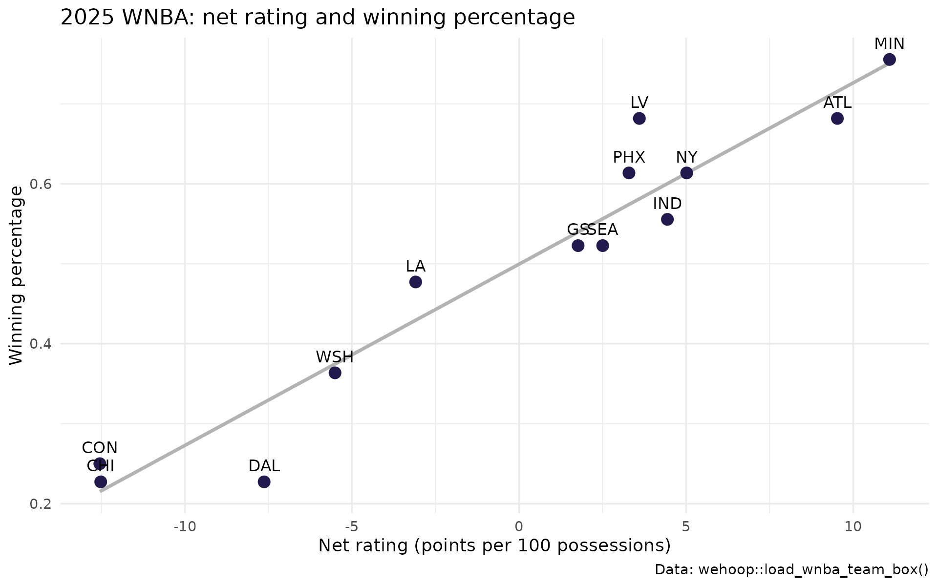

Scatter plot of 2025 WNBA teams with net rating on the x-axis and winning percentage on the y-axis.

cor(team_season$net, team_season$win_pct)
#> [1] 0.9611032

The four factors

Dean Oliver identified four things that decide most games, each measured for a team’s offense and the same quantity allowed on defense:

Factor	Offense	Defense
Shooting	$\text{eFG\%} = \frac{\text{FGM} + 0.5 \times \text{3PM}}{\text{FGA}}$	the opponent’s eFG%
Turnovers	$\text{TOV\%} = \frac{\text{TOV}}{\text{Poss}}$	the opponent’s TOV%
Offensive rebounding	$\text{OREB\%} = \frac{\text{OREB}}{\text{OREB} + \text{Opp DREB}}$	$\text{DREB\%} = \frac{\text{DREB}}{\text{DREB} + \text{Opp OREB}}$
Free throws	$\text{FT rate} = \frac{\text{FTM}}{\text{FGA}}$	the opponent’s FT rate

Some sources define FT rate as FTA / FGA, which measures getting to the line rather than converting there. Oliver’s version, FTM / FGA, is used below.

four_factors <- team_season |>
  mutate(
    efg = (fgm + 0.5 * fg3m) / fga,
    tov_pct = tov / poss,
    oreb_pct = oreb / (oreb + opp_dreb),
    ft_rate = ftm / fga,
    opp_efg = (opp_fgm + 0.5 * opp_fg3m) / opp_fga,
    opp_tov_pct = opp_tov / poss,
    dreb_pct = dreb / (dreb + opp_oreb),
    opp_ft_rate = opp_ftm / opp_fga
  ) |>
  select(team, net, efg, tov_pct, oreb_pct, ft_rate,
         opp_efg, opp_tov_pct, dreb_pct, opp_ft_rate) |>
  arrange(desc(net))

four_factors |>
  mutate(across(-team, ~ round(.x, 3)))
#> # A tibble: 13 × 10
#>    team     net   efg tov_pct oreb_pct ft_rate opp_efg opp_tov_pct dreb_pct
#>    <chr>  <dbl> <dbl>   <dbl>    <dbl>   <dbl>   <dbl>       <dbl>    <dbl>
#>  1 MIN    11.1  0.539   0.163    0.259   0.179   0.481       0.193    0.74 
#>  2 ATL     9.53 0.514   0.157    0.267   0.216   0.478       0.153    0.798
#>  3 NY      5.02 0.526   0.17     0.208   0.239   0.483       0.168    0.736
#>  4 IND     4.44 0.516   0.172    0.264   0.201   0.501       0.187    0.757
#>  5 LV      3.60 0.506   0.161    0.235   0.225   0.489       0.168    0.745
#>  6 PHX     3.29 0.502   0.166    0.244   0.203   0.486       0.185    0.755
#>  7 SEA     2.50 0.505   0.15     0.199   0.178   0.497       0.197    0.742
#>  8 GS      1.77 0.482   0.181    0.26    0.23    0.472       0.163    0.76 
#>  9 LA     -3.09 0.521   0.181    0.241   0.234   0.524       0.163    0.736
#> 10 WSH    -5.51 0.483   0.19     0.235   0.245   0.505       0.17     0.776
#> 11 DAL    -7.63 0.469   0.168    0.276   0.206   0.531       0.163    0.757
#> 12 CHI   -12.5  0.476   0.211    0.291   0.198   0.521       0.148    0.747
#> 13 CON   -12.5  0.458   0.173    0.244   0.216   0.53        0.184    0.726
#> # ℹ 1 more variable: opp_ft_rate <dbl>

Which factor tracks winning most closely this season? Correlate each team’s factor margin (offense minus what it allowed) with net rating. With only 13 teams this is descriptive, not a model.

four_factors |>
  transmute(
    net,
    shooting = efg - opp_efg,
    turnovers = opp_tov_pct - tov_pct,
    rebounding = oreb_pct - (1 - dreb_pct),
    free_throws = ft_rate - opp_ft_rate
  ) |>
  summarise(across(-net, ~ cor(.x, net))) |>
  tidyr::pivot_longer(everything(), names_to = "factor_margin", values_to = "cor_with_net")
#> # A tibble: 4 × 2
#>   factor_margin cor_with_net
#>   <chr>                <dbl>
#> 1 shooting            0.954 
#> 2 turnovers           0.552 
#> 3 rebounding         -0.0274
#> 4 free_throws         0.388

Signs are arranged so that a positive margin is good for the team in every row.

Player efficiency: eFG%, TS% and usage

True shooting percentage folds free throws into shooting efficiency. Each true shot attempt is a field goal attempt or a free throw trip (0.44 of an FTA):

$\text{TS\%} = \frac{\text{PTS}}{2 \times (\text{FGA} + 0.44 \times \text{FTA})}$

Usage rate is the share of team possessions a player finishes, by a shot, a trip to the line or a turnover, while she is on the court:

$\text{USG\%} = 100 \times \frac{(\text{FGA} + 0.44 \times \text{FTA} + \text{TOV}) \times (\text{Team MIN} / 5)} {\text{MIN} \times (\text{Team FGA} + 0.44 \times \text{Team FTA} + \text{Team TOV})}$

Usage needs the team totals from the games the player played, so join each player-game to its team-game row first.

team_game_totals <- games |>
  select(game_id, team_id, team_min, team_fga = fga, team_fta = fta, team_tov = tov)

players <- player_box |>
  filter(did_not_play == FALSE, !is.na(minutes), minutes > 0) |>
  inner_join(team_game_totals, by = c("game_id", "team_id")) |>
  group_by(athlete_display_name, team_abbreviation) |>
  summarise(
    games = n(),
    min = sum(minutes),
    pts = sum(points),
    fga = sum(field_goals_attempted), fgm = sum(field_goals_made),
    fg3m = sum(three_point_field_goals_made),
    fta = sum(free_throws_attempted),
    tov = sum(turnovers),
    team_min = sum(team_min),
    team_used = sum(team_fga + 0.44 * team_fta + team_tov),
    .groups = "drop"
  ) |>
  mutate(
    efg = (fgm + 0.5 * fg3m) / fga,
    ts = pts / (2 * (fga + 0.44 * fta)),
    usage = 100 * (fga + 0.44 * fta + tov) * (team_min / 5) / (min * team_used)
  )

players |>
  filter(min >= 500) |>
  arrange(desc(usage)) |>
  select(athlete_display_name, team_abbreviation, games, min, pts, efg, ts, usage) |>
  head(12)
#> # A tibble: 12 × 8
#>    athlete_display_name team_abbreviation games   min   pts   efg    ts usage
#>    <chr>                <chr>             <int> <dbl> <int> <dbl> <dbl> <dbl>
#>  1 A'ja Wilson          LV                   40  1248   937 0.524 0.596  31.7
#>  2 Shakira Austin       WSH                  38   874   481 0.467 0.506  29.4
#>  3 Satou Sabally        PHX                  39  1040   636 0.469 0.533  28.7
#>  4 Napheesa Collier     MIN                  34  1099   767 0.571 0.627  28.5
#>  5 Sabrina Ionescu      NY                   38  1191   693 0.472 0.537  28.3
#>  6 Tina Charles         CON                  43  1225   700 0.449 0.515  28.0
#>  7 Kahleah Copper       PHX                  28   752   438 0.503 0.548  27.3
#>  8 Kelsey Mitchell      IND                  45  1418   902 0.533 0.570  27.2
#>  9 Breanna Stewart      NY                   31   948   566 0.487 0.570  26.8
#> 10 Brittney Sykes       WSH                  25   774   385 0.412 0.498  26.2
#> 11 Marina Mabrey        CON                  35  1103   504 0.434 0.477  25.6
#> 12 Courtney Williams    MIN                  45  1296   610 0.474 0.493  25.5

qualified <- players |> filter(min >= 500)

ggplot(qualified, aes(usage, ts)) +
  geom_point(alpha = 0.6, color = "#7c689c") +
  geom_text(
    aes(label = athlete_display_name),
    data = qualified |> filter(usage > quantile(usage, 0.93) | ts > quantile(ts, 0.97)),
    size = 3, vjust = -0.8, check_overlap = TRUE
  ) +
  scale_y_continuous(labels = scales::percent) +
  labs(
    title = "2025 WNBA: usage and true shooting (500+ minutes)",
    x = "Usage rate (%)", y = "True shooting",
    caption = "Data: wehoop::load_wnba_player_box(), wehoop::load_wnba_team_box()"
  ) +
  theme_minimal()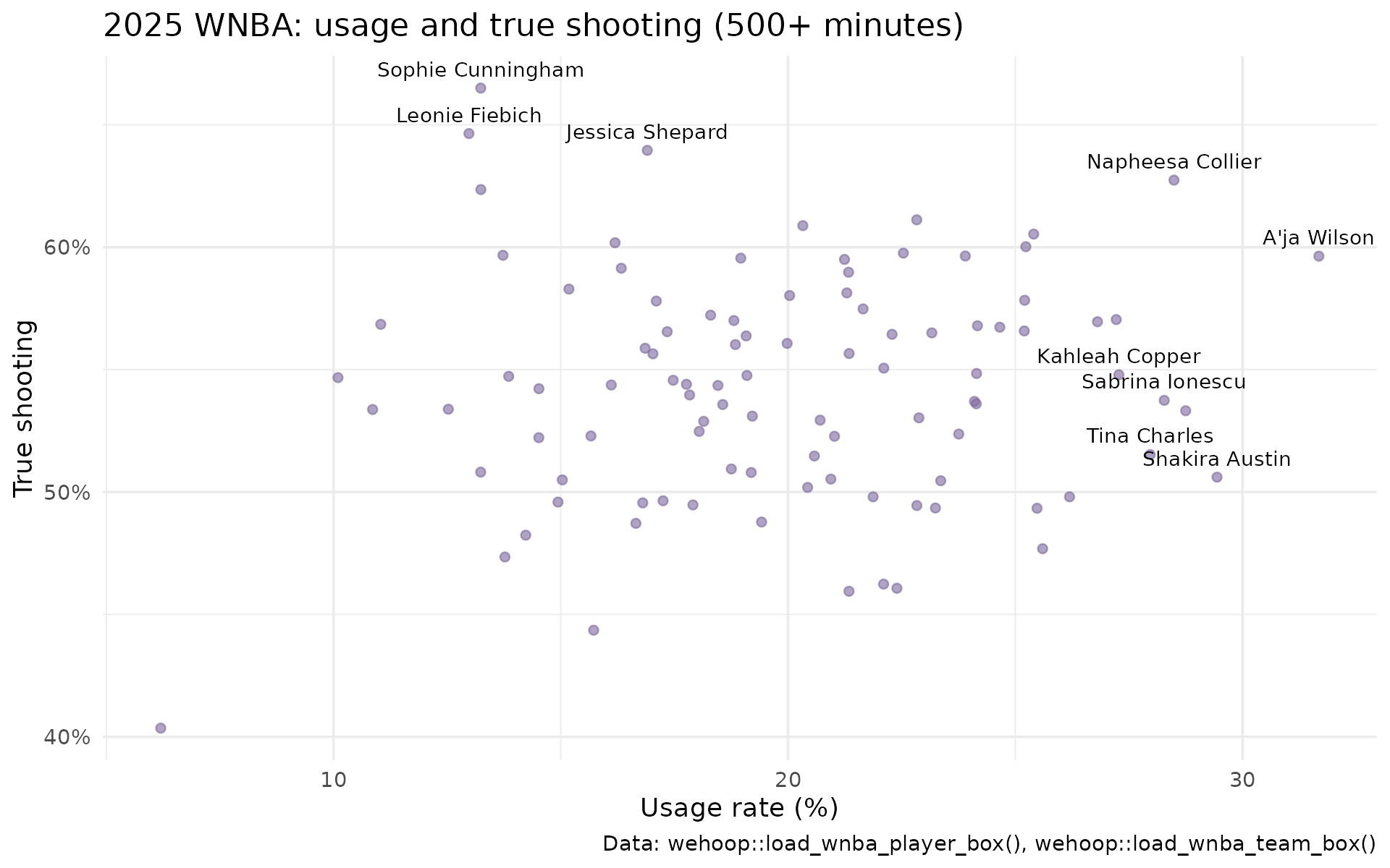

Scatter plot of 2025 WNBA players with at least 500 minutes, usage rate on the x-axis and true shooting percentage on the y-axis.

Players in the top-right carry a large share of the offense and stay efficient, which is hard to sustain.

Women’s college basketball

The college box scores have the same columns, so the code carries over. Division I teams also play non-Division I opponents, so restrict the table to teams with a full schedule in the release.

wbb_box <- load_wbb_team_box(seasons = 2026) |>
  filter(season_type %in% c(2, 3))

wbb_games <- wbb_box |>
  transmute(
    game_id, team_id, team = team_location, team_score,
    fga = field_goals_attempted, fgm = field_goals_made,
    fg3m = three_point_field_goals_made, fta = free_throws_attempted,
    oreb = offensive_rebounds, tov = total_turnovers,
    poss = fga - oreb + tov + 0.44 * fta
  )

wbb_games <- wbb_games |>
  inner_join(wbb_games |> select(game_id, opp_team_id = team_id,
                                 opp_score = team_score, opp_poss = poss),
             by = "game_id", relationship = "many-to-many") |>
  filter(team_id != opp_team_id)

wbb_games |>
  mutate(avg_poss = (poss + opp_poss) / 2) |>
  group_by(team) |>
  summarise(
    games = n(),
    ortg = 100 * sum(team_score) / sum(avg_poss),
    drtg = 100 * sum(opp_score) / sum(avg_poss),
    efg = (sum(fgm) + 0.5 * sum(fg3m)) / sum(fga),
    .groups = "drop"
  ) |>
  filter(games >= 25) |>
  mutate(net = ortg - drtg) |>
  arrange(desc(net)) |>
  head(10)
#> # A tibble: 10 × 6
#>    team                games  ortg  drtg   efg   net
#>    <chr>               <int> <dbl> <dbl> <dbl> <dbl>
#>  1 UConn                  39  119.  69.3 0.585  50.1
#>  2 LSU                    35  122.  78.5 0.548  43.5
#>  3 UCLA                   38  122.  81.8 0.565  39.8
#>  4 Texas                  39  116.  77.2 0.528  39.0
#>  5 South Carolina         40  117.  79.2 0.546  38.0
#>  6 TCU                    38  109.  81.0 0.540  28.4
#>  7 North Dakota State     34  114.  87.1 0.531  27.1
#>  8 Fairfield              33  109.  81.7 0.547  26.8
#>  9 Fairleigh Dickinson    35  107.  80.1 0.498  26.4
#> 10 Michigan               35  109.  83.2 0.512  26.1

These are raw ratings: they do not account for who a team played. A team that beats weak opponents by 40 looks better here than it is. The team ratings model adjusts for schedule strength.

Official numbers for a single game

The WNBA Stats API publishes its own advanced box scores per game, computed from counted possessions. They make a useful check on your formulas. These are live calls to stats.wnba.com, so they are not run here.

wnba_boxscorefourfactorsv3(game_id = "1022500001")
wnba_boxscoreadvancedv3(game_id = "1022500001")
wnba_boxscoreusagev3(game_id = "1022500001")

Where to go next

Shot charts: where the shots behind eFG% come from.
WNBA player impact model: RAPM, box plus/minus and WAR, which go beyond per-possession box score rates.
Women’s college team ratings model: opponent-adjusted efficiency.
Women’s college player value model: a box plus/minus built from these per-100 rates.
The release loaders in the function reference.

Saiem Gilani, Geoffery Hutchinson